Before starting my role as an external auditor, I did not expect to use Microsoft Excel in my job as much as I do (almost daily). Excel is used to document the majority of testing from the audit side. However, our clients within the finance team also tend to use Excel for their own calculations and workings. It therefore really does help to be Excel proficient as a finance professional. If you are a new joiner, this blog is a great place to start. That being said, there are some Excel tips and tricks that I only picked up fairly recently too. Hopefully this article has something for everyone or boosts your confidence if you are an Excel wiz.
Note: I will assume you have the basic understanding of using Excel such as “=SUM(…“, freeze panes, filtering, sorting data, etc so will skip these.
If you do prefer watching to reading and want to see live demos of these tips, click here for the YouTube video!
1) Pivot Tables
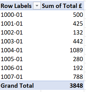
Starting off with the classic pivot tables, I first came across these when I was working as a business analyst at IBM. Pivot tables are extremely, extremely useful where you have hundreds or thousands of rows/columns of raw data. For example, an Excel spreadsheet with every single financial transaction for the current financial year. What a pivot table allows you to do is to extract the exact data you need from the raw data. Within seconds I could find out the total amount posted to an account code each quarter.

A basic tutorial can be found here. Key points/Excel tips I would make is:
- Make sure there are no blank fields/columns when creating the pivot table
- You can refresh pivot tables if the raw data changes
- I would highly recommend playing around with a pivot table to improve and get quicker at creating these how you need
- You may find when you drag and drop fields into the pivot areas that the value is sometimes automatically set to “count”; instead of giving the total value it tells you the total number of entries. To correct this simply click on the dropdown option where it states “count of…”, select “value field settings…”, select “sum” and “OK”.
- Copying and pasting values of the pivot data can be especially useful where you want to sort the data and play around with it further
- Always remember the grand total is given at the bottom as well as “(blank)” data.
2) VLOOKUP
This is arguably one of the most important functions to be aware of. I remember first coming across the VLOOKUP function during my ICT GCSE. I of course did not remember much by time I actually needed to use it in a work scenario but it definitely would have helped!
If you are unaware of this function, to put it simply, the VLOOKUP allows you to match data from different sources. You do need one unique field that is included in both datasets to match these up. For example, imagine you have a list of customers where one list includes details of the total revenue and the customer address but the customers are ordered randomly. A VLOOKUP would allow you to match by customer the total revenue and address so you can see all this data in one place. The unique field in this example could be customer name or customer number.

Here is a tutorial for performing VLOOKUPs. My Excel tips for this are:
- The brutal “#N/A” can mean one of three things. Firstly, that there is an error in your VLOOKUP formula. It could also mean that the item you are looking for is missing from the data (Ctrl + F and doing a quick find will help clarify if this is the case). Finally in the unlikely scenario, “#N/A” may be pulled correctly from the data.
- Make sure your data is formatted correctly! If your raw data which you are using to do the match, such as customer number is in text format but the other data source is in number it may not work.
- A common reason for the VLOOKUP not working is because there is a hidden space before or after the lookup value.
- When dragging down the function into the cells below, make sure you have used “$” for the table array cells e.g. “$D$5:$F$50”. Otherwise you will start to lose the data from the top of the table array and it will not get matched!
3) Data Formatting
If you ever receive very messy data in a format you are not comfortable with using, there are several options available to you:
- Delete blank rows – click here
- Text to columns allows you to split one cell of data into several – click here
- There are Excel Add-ins that can help with this too. For example, within my firm we have access to an Excel Analytics toolbar. This has many useful features such as the import wizard. Although it is complicated to use initially, it can be very useful once you get the hang of it.
- Removing duplicates – if the data has many rows with the same information, you can remove duplicates as explained here or see the method I prefer here.
4) Quick Access Toolbar
This Excel tip is extremely simple and self explanatory. If you want to be able to access buttons quickly, such as filter, format painter, etc as can be seen below, you can add these too your quick access toolbar. These will always be at the top of your Excel file.

You can find out how to do this and tailor it for yourself here. It really does save me so much time when using Excel and is a nice little Excel tip if I do say so myself.
5) Absolute Function
This is one that many may already be aware of and it may seem quite obvious. I will state it anyway just in case. If you want to turn negative values into positives, instead of “=(cell*-1)” you can use the “=ABS(…” function. It is quick and easy and can of course be dragged down from the bottom right corner to apply to all in a column/row.
I will add another quick Excel tip here that is somewhat related. If you wanted to identify items that net off you could turn these all into absolute figures and then identify duplicates as mentioned above. Another option is to sort the absolute value column from smallest to largest for example.
6) Other Useful Functions
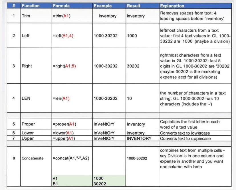
Here is pretty much a function dump. I came across this photo a few weeks ago shared by @thebig4accountant on Instagram and thought it was a good one to include. I cannot say I use these but they may help you.

7) Adjusting Rows
This one may seem obvious but I do not actually think many are aware of this. If you want to adjust a column/row size, the general approach is to adjust this by sliding the boundary individually for each column/row. However, you can actually do this for the whole workbook at once. Highlight all columns/rows you want to adjust whilst you adjust one as normal and you should find every column/row is adjusted to that same size.
8) Drop-Down Lists
In all honesty, I really do not use this all too often but when you want data to be provided in a certain way keeping errors to a minimum, drop-down lists are the way forward. To create this you simply need to select “data validation” from the “data” tab and create the list through cell references. Click here for a tutorial that actually takes it a few steps further and creates a dependent drop-down list.
9) Fix Slow Loading Excel Files
So this is something you may not need to use very often but it is actually pretty useful. I have had instances where I have been sent an Excel file that for some reason takes a very long time to load. The reason behind this could be because there are lots of different formulas updating in the background. I have actually found a good blog that explains this further and how to address this issue.
10) Excel Shortcuts
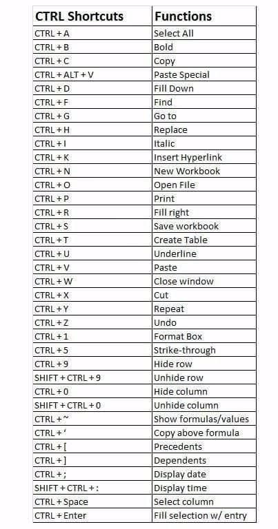
Now this is where it gets exciting and the real Excel wizards come out. Admittedly I honestly am still pretty much an amateur but I love how many Excel shortcuts there are. I will show you some of the possibilities below. Following this, besides the obvious such as “ctrl+c” and “ctrl+v”, I will talk you through the ones I use the most.

My Favourite Excel Shortcuts
From the above, I recently learnt the “ctrl + [“ shortcut and it honestly is a lifesaver. The above table states “precedents” and I would literally scan over that and think it would not help me. However, it is an extremely useful shortcut particularly where you are working with a lot of formulas. This shortcut allows you once you have clicked into a cell with a formula to follow the formula and find out exactly where the numbers have come from. For example, if the cell includes “=(C18*11)” and you use this shortcut when clicking on this formulated cell, it will take you to cell C18 to show you exactly where it is from.
Another useful shortcut not mentioned above is “ctrl + shift + +”. That looks odd but you are meant to press the “+” key at the end. This is a shortcut to add rows/columns. Simply highlight the row/column you want to insert the row/column ahead of, input the shortcut and there is your newly inserted row/column.
The next shortcut is one I shared with a client who was very grateful for my time by the end of the meeting. This is “ctrl + down arrow”. This will take you right to the bottom cell of a row so you do not need to scroll all the way down. This could equally work with the up, left or right arrows. If you throw shift into the mix with “ctrl + shift + down arrow”, it will highlight all the cells to the bottom of the row.
The final I will share is “alt + tab”. I never use this but this is the one to flick between different (Excel) files you have open and this is how to really look like you are a quick Excel wizard.

Excel Tips and Tricks Summary
Hopefully there was at least one good Excel tip or trick in here that you can takeaway with you. Like I said, I am by no means a pro and I too have much more to learn. If you do ever find yourself struggling with Excel you can usually Google and find what you are looking for within 0.25 seconds.
If you found this blog helpful, feel free to buy me a coffee or join my journey for more!


[…] to slow you down and so I would suggest getting better at using Excel sooner rather than later. This blog will definitely help. If there is anything else you are unsure of when using Excel, Google is […]